3. MODEL DEVELOPMENT

3.1 Model Conceptualization, Assumptions, and Limitations

Any mathematical model involves a simplification of real-world systems with the degree of simplification being inversely proportional to the sophistication of the model. Simpler models require more significant idealization of the real-world system. The Vadose-Groundwater Model (VG Model) is a relatively simple model intended primarily for screening contaminant level estimation within the solute transport phenomena in the subsurface. In this section, the assumptions and limitations are separately discussed for the vadose zone and saturated zone modules.

3.1.1 Vadose Zone Leaching

The movement of an organic contaminant in the vadose zone can be described within and among three different phases: (1) as a solute dissolved in water, (2) as a gas in the vapor phase, and (3) as an adsorbed compound in the solid phase (see Figure 2.2). Equilibration among the phases occurs according to distribution coefficients defined by the user. Contaminant decay was incorporated in the model assuming a uniform decay rate for the three different phases of the user selected chemical. The first part (vadose zone leaching) of the VG model simulates vertical transport through vertically heterogeneous soil layers by advection and dispersion in the liquid phase and by gaseous diffusion in the vapor phase.

These processes are conceptualized as occurring in a number of distinct, user-defined soil columns, which are vertically divided into a series of user-defined cells within each layer. The soil columns and layers may differ in soil properties, recharge rate, and depth to water. Within each soil column heterogeneous conditions are assumed due to differences in soil properties among different geologic layers and also in contaminant concentration (see Figure 3.1). During each time step intervals the migration of the contaminant through each cell in the soil column is calculated. Hence, the first part of the VG model can account for heterogeneity both laterally and vertically. The numbers of columns and layers employed in the simulation have a mathematical capability of 50 and 1000, respectively.

Figure 3.1 Schematic diagram illustrating the discretization of soil columns in vadose zone and the saturated zone mixing aligned parallel to groundwater flow direction.

Contaminant transport processes in the subsurface are simulated after the first part of the VG model has calculated contaminant equilibrium concentration in the liquid and vapor phases based on the user provided initial solid-phase concentration [mg/Kg]. Calculations of advective and dispersive transport of contaminants in solution are based on the assumed parameter values. The advective vapor flow in the soil is assumed to be small and is therefore neglected. Therefore, contaminants in the vapor phase diffuse between adjacent cells based upon the calculated concentration gradients. After contaminants have equilibrated among three phases, the total mass in each cell is calculated. These steps are conducted for each selected time interval, and each soil column is simulated independently assuming no horizontal mass transfer between columns.

For computational purposes each soil column is divided into a series of cells. When developing a model simulation, it is important to fully understand the implications of the first part of the VG model conceptualization. The following assumptions are made in the conceptualization of the first part of the VG model in the vadose zone.

1. Linear isotherms describe the partitioning of the pollutant among the liquid, vapor, and solid phases. Local or instantaneous equilibrium among these phases is assumed within each cell in every layer.
2. Liquid phase dispersion and vapor phase diffusion are included. In the model the two terms are combined as one via the Henry's equilibrium constant.
3. Unless there is a special remedial action such as soil venting, vapor flow in the subsurface is negligible. Although some researchers (Falta et al., 1988) have found that density driven advective flow in the soil is also an important mechanism for gas movement, the vapor-phase advection is assumed as negligibly small compared to the infiltrating water velocity and omitted in this screening level model.
4. Organic contaminants, especially hydrocarbons, generally undergo some degree of degradation in the vadose zone. The module uses two decay constants to describe the first order decay; one for the contaminant decay in the soil, and another for the contaminant source reduction. The finite initial source concentration decreases due to either degradation or flushing by fresh water infiltration.
5. There is no capillary fringe. In most permeable soils this is very small in proportion to the column length and can be neglected.

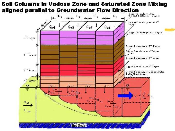
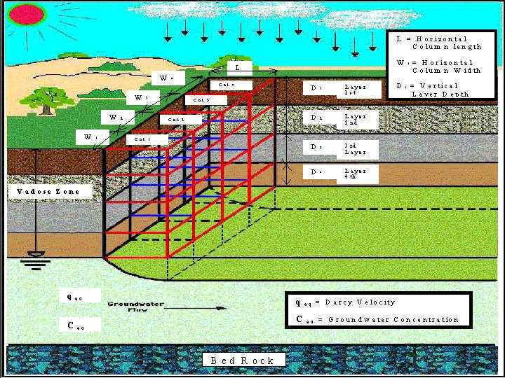
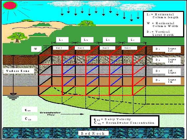
3.1.2 Saturated Zone Mixing

The leachate from the vadose zone will reach groundwater in the saturated zone and will be mixed. In the second part (saturated zone mixing) of the VG model, this mixing process is simulated by employing a mass-balance principle.

For the purpose of mixing calculation in the saturated zone, the conceptual vadose zone soil columns are assumed to be arranged in one of two ways. To represent a contaminant source in the soil, a group of vertical soil columns can be arranged at either transverse or parallel alignment to the groundwater flow direction (see Figures 3.2 and 3.3). For the transverse arrangement (Figure 3.2), each soil column is treated independently both in the vadose and in the saturated zones. For the parallel case (Figure 3.3), only the vadose zone migration in each column is treated independently. For the saturated zone mixing, for the parallel case, the up-gradient mixed concentration is used as influent concentration for estimating the next down-gradient column's concentration. In both cases, the bottom of each soil column is assumed to be parallel to the water table.

Figure 3.2 Schematic diagram illustrating model conceptualization as soil columns in the vadose zone and the mixing zone in the saturated medium. The soil columns are arranged transverse to the groundwater flow direction.

Figure 3.3 Schematic diagram illustrating conceptualization as soil columns in the vadose zone and the mixing zone in the saturated medium. The soil columns are arranged parallel to groundwater flow direction.

For the screening level mixing calculation, the following assumptions are made in the development of the second part of the VG model.

1. The leachate is assumed to be completely mixed in the aquifer directly under the soil column.
2. The aquifer is homogeneous with steady state and uniform groundwater flow.
3. Groundwater mounding due to potential high infiltration is neglected.
4. The decay of the solute in the saturated zone is conservatively assumed to be small and negligible.
5. The leachate penetration in the aquifer is estimated using the relationship presented in EPACML (EPA, 1990a). It is introduced as a function of the vertical infiltration velocity, horizontal length of the source in the soil column, vertical transverse dispersivity in the aquifer, horizontal groundwater velocity, and the aquifer thickness. When the estimated penetration is greater than the thickness of the aquifer, the value is set as equal to the thickness of the aquifer.
6. Contaminant spreading in the horizontal transverse direction (i.e., perpendicular to the groundwater flow) is neglected. This assumption may cause a somewhat higher mixed concentration than would occur naturally.

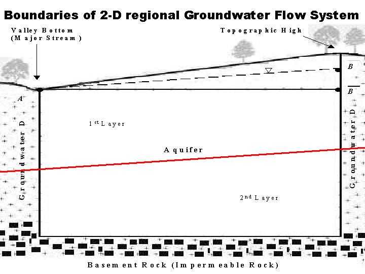
3.1.3 Groundwater Flow System

Groundwater flow models involving Laplace's equation and suitable boundary conditions are described by Toth (1962). He was able to draw conclusions about the configuration of regional groundwater systems by using a mathematical model. Figure 3.4 represents a cross section through a small watershed bounded on one side by a topographic high, which marks a regional groundwater divide, and on the other side by a major stream, which is a groundwater discharge area and marks another regional groundwater divide. The aquifer is assumed to consist of heterogeneous, isotropic, porous material underlain by impermeable rock.

Figure 3.4 Schematic representation of the boundaries of a two dimensional regional groundwater flow system.

The left and right groundwater divides can be represented mathematically as impermeable, no-flow boundaries. Although no physical barrier exists, a groundwater divide has the same effect as an impermeable barrier because no groundwater crosses it. Groundwater to the right of the valley bottom discharges at point A, and groundwater on either side of the topographic high flows away from point B. The lower boundary is also a no-flow boundary because the impermeable basement rock forms a physical barrier to flow. The upper boundary of the mathematical model is the horizontal line A even through the water table of the physical system lies above A . Thus this regional problem domain of the mathematical model is an approximation to the actual shape of the saturated flow region. Along the boundary A, the head is taken to be equal to the height of the water table, and the water table configuration is considered to be a straight line.

In an undeveloped watershed, the fluctuations of the water table position can assume that the system is at a steady state on an annual basis, usually the U.S. Geological Survey water year (1 October to 30 September). The water table position at the beginning of the year is the same as the position at the end of the year; there was no net accumulation or loss of water from the system, viz, storage change.

3.2 Theoretical Background

In this section, a brief theoretical development of the Vadose-Groundwater model (VG model) is presented for vadose zone transport, saturated zone mixing, and groundwater flow net.

3.2.1 Vadose Zone Transport

If we consider three equilibrium phases of pollutants in an unsaturated soil column, its one-dimensional heterogeneous governing transport equation is expressed as follows:

where C_w is concentration of a contaminant in liquid (water) phase [mg/L]. C_a is concentration of a contaminant in vapor (air) phase [mg/L]. C_s is concentration of a contaminant in solid phase [mg/Kg]. q_w is volumetric water content (volume of water / total volume) [ft³/ft³]. q_a is air-filled porosity (volume of air / total volume) [ft³/ft³]. Note that the total porosity n equals the sum of water filled porosity and air filled porosity. q_w is water flow velocity (recharge rate) [ft/yr]. The air flow velocity (q_a) is assumed to be zero in this study. D_w is dispersion coefficient for the liquid phase contaminant in the pore water [ft²/yr]. D_a is gaseous phase diffusion coefficient in the pore air [ft²/yr]. m_w is first order decay rate of a contaminant in water phase [1/yr]. m_a is first order decay rate of a contaminant in gaseous phase [1/yr]. m_s is first order decay rate of a contaminant in solid phase [1/yr]. In this model, for simplicity, it is assumed that m_w = m_a = m_s = m. r_b is bulk density of the soil [gr/cm³]. z is vertical coordinate with positive being downward. t is time [yr].

Instantaneous equilibrium (partitioning) of the contaminant among the phases is assumed to be realized according to the following linear relationships:

Liquid-solid phase equilibrium is

Liquid-gas phase equilibrium is

where K_d [ml/g] is the distribution coefficient between the solid phase and liquid phase, and H (H = K_H /(RT), [dimensionless]) is the partition coefficient between the air phase and water phase. Using the empirical relationship, K_d can be expressed as K_d = K_oc·f_oc, where K_oc [ml/g] is the organic carbon-water partition coefficient and f_oc [g/g] is the fraction organic carbon of the soil.

The dimensionless form of the Henry's partition coefficient, H, can be determined from the more common form having the units of atmospheres-cubic meters per mole [atm-m³/mol] using the following equation

where K_H [atm-m³/mol] is the dimensional form of Henry's Law constant, R is the universal gas constant (R = 8.2 · 10^-5 [atm-m³/mol·K]), and T is the absolute temperature [°K = 273.16 + °C].

The dispersion coefficient, D_w, in the unsaturated zone is regarded as a linear function of the pore water velocity as the equation (2.13). The scale-dependent dispersivity is the equations (2.14) and (2.15).

The equations (2.14) and (2.15) can be rewritten for the English unit as:

It should be recognized that dispersion remains a significant uncertainty in the modeling effort. Considerable debate exists regarding the appropriate practical treatment of field-scale dispersion. In general, field tests are the only methods by which reasonable estimates for dispersion can be obtained.

The gas phase diffusion coefficient (D_a) in the porous medium is calculated by modifying the free air diffusion coefficient using the Millington model (Millington, 1959):

where D_air is the diffusion coefficient of the contaminant in the free air, and n is the total porosity of the soil.

By substituting equation (3.2) and (3.3) into (3.1), and neglecting the air flow velocity (q_a = 0), the governing transport equation can be simplified as:

If we set as

By substituting equations (3.9) and (3.10) into (3.8)

The equation (3.11) can be rewritten as:

Initial and Boundary Conditions

To solve equation (3.12), initial and boundary conditions are required as follows.

where C_s(z,0) is the initial solid-phase concentration specified by the user. When the distribution coefficient (K_d = K_oc· f_oc) is zero, liquid-phase concentration must be entered as an initial concentration to avoid the program run-time error (division by zero).

The most common type of boundary condition to be applied at the top of the soil column is either the first type (Dirichlet's) or the third type (Cauchy's) as shown below.

or

where C₀ is the liquid phase solute concentration in the infiltration water, g is the decay rate [1/yr] of the solute source due to either degradation or flushing by the infiltration, and t₀ is the duration of solute release [yr] which can be selected to simulate continuous input.

At the bottom of the soil column, the second type boundary condition (Neuman's) is applied.

In applying this boundary condition, equation (3.19) is actually implemented at a finite column length (i.e., z is not infinity). To reduce the finite length effect, dummy cells are added at the bottom of the soil column automatically in the numerical calculation in the model. After evaluation of C_w(z,t), the total contaminant mass per unit volume of the soil is calculated as:

3.2.2 Saturated Zone Mixing

After estimating the liquid phase solute concentration (C_w) at the bottom of the soil column, the mixed concentration in the aquifer can be calculated using a mass-balance technique as below (USEPA, 1989; Summers et al., 1980):

where C_aq is the concentration of horizontal groundwater influx, q_aq is the Darcy velocity in the aquifer, A_aq is the cross-sectional aquifer area perpendicular to the groundwater flow direction, and A_soil is the cross-sectional area perpendicular to the vertical infiltration in the soil column. The aquifer area (A_aq) is determined by multiplying the horizontal width of the soil column with the vertical solute penetration depth.

As discussed in Section 3.1.2, Saturated Zone Mixing, the procedure for the mixing calculation is different depending on the type of soil column arrangement. In the case of the transverse (right angle) arrangement, the mixing calculation is straight forward: simply apply equation (3.21) at each mixing element underneath the soil columns. For the parallel arrangement case, however, the mixed concentration at the upgradient cell is considered as an influx concentration to the next cell (see Figure 2.3). The mixing concentration at the next cell is estimated by re-applying equation (3.21) using the two inflow concentrations: one from the effluent from the upgradient cell and the other from the leaching from the soil column.

Solute Penetration Depth

The solute penetration depth is the mixing thickness of the contaminant in the aquifer beneath the soil column. An estimation of the plume thickness in the aquifer can be made using the relationship below (adapted from USEPA, 1990a):

where, H_d is the penetration depth [ft], a_v is the transverse (vertical) dispersivity [ft] of the aquifer, L is the horizontal length dimension of the waste [ft], and B is the aquifer thickness [ft]. In equation (3.22) the first term represents the thickness of the plume due to vertical dispersion and the second term represents that due to displacement from infiltration water. When implementing this relationship, it is necessary to specify that in the event the computed value of H_d is greater than B, the penetration thickness, H_d is set equal to B (USEPA, 1990a).

Assumptions and Limitations Associated with the Penetration Depth Estimation

The method introduced in equation (3.22) is based on two major assumptions (refer to Appendix D for its derivation) and, therefore, has subsequent limitations. First, in estimating the dispersive penetration depth, there are two dispersion components in the mixing zone: one from the transverse (z-directional) dispersion by the horizontal groundwater velocity, and the other from the longitudinal (z-directional) dispersion by the infiltration velocity. In the first term of equation (3.22), however, the longitudinal dispersion due to infiltration is neglected by assuming that the horizontal groundwater velocity is much greater than the infiltration velocity. Therefore, when the horizontal groundwater velocity is not substantially greater than the vertical infiltration velocity, the equation underestimates the penetration depth and overestimates the mixed concentration.

Secondly, the second term in equation (3.22), the advective penetration depth due to infiltration, is based on the assumption that the vertical (infiltration) velocity varies linearly with aquifer depth, with a maximum value at the top of the water table (i.e., at the bottom of the soil column) and zero at the bottom of the aquifer. In case of either large aquifer thickness or higher horizontal velocity compared to the vertical, the vertical component of groundwater velocity becomes zero before the infiltration water reaches the bottom of the aquifer. In this case, the equation (3.22) overestimates penetration depth and, subsequently, underestimates the mixed concentration.

Due to the assumptions and limitations discussed above, the user must be careful when using the equation (3.22). Whenever field data are available, the measured solute penetration depth should be used instead of the equation. Otherwise, the input parameter values must be checked to see whether the assumptions are valid. For example, compare the horizontal and vertical groundwater velocities to ensure the horizontal velocity is much larger than the vertical one (e.g., 10 times greater). In the second part of the VG program, an option is provided to choose either the measured penetration depth or to estimate the depth based on the aquifer parameter values.

Adjustment of the Estimated Penetration Depth

No adjustment of the penetration depth is required when either the depth is measured in the field or the soil columns are arranged at right angle to the horizontal groundwater flow direction. For the parallel arrangement, however, when the penetration depth needs to be estimated by the equation (3.22), the estimated depth is adjusted as follows. As shown in the example (Fig. 2.3), the total source dimension (L) is subdivided into four segments (L₁ through L₄) and the penetration depth for each soil column is calculated as:

where the subscript i represents column 1 through 4. Since the relationship between L and H_d is not linear in the equations (3.22 and 3.23), the sum of individual penetration depths based on the segment length is different from the overall penetration depth (i.e., H_d  H_d1 + H_d2 + H_d3 + H_d4). Note that the overall penetration depth (H_d) is based on the total contaminant length dimension (L) and the arithmetic average values of a_v, B, q_aq and q_w for all columns. Therefore, the individual penetration depth is adjusted as:

where is the adjusted penetration depth for each column.

Consequently, the relationship between the adjusted and individual penetration depth is expressed as:

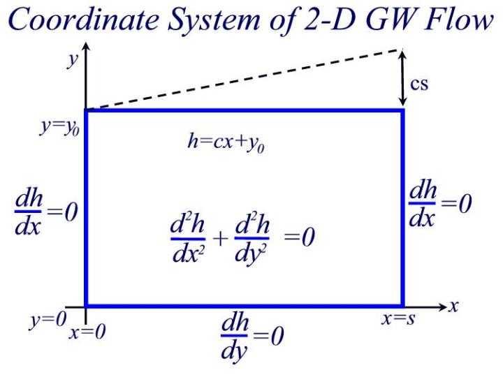
3.2.3 Groundwater Flow System

Governing Equation and Visualization

The two-dimensional generalization of Darcy's law requires that the one-dimensional form be true for each of the x and y components of flow as the equations (2.17) and (2.18). The two-dimensional continuity equation for steady-state conditions is equation (2.19). Laplace's equation combines Darcy's law and the continuity equation into a single second-order partial differential equation. Darcy's law, equations (2.17) and (2.18), is substituted component by component into equation (2.19) to give the equation (2.20). If we assume horizontal hydraulic conductivity is much bigger than vertical hydraulic conductivity and constant, then equation (2.20) becomes equation (2.21) and the hydraulic conductivity in this governing equation is horizontal hydraulic conductivity, K.

Toth (1962) assumed that, in an undeveloped watershed, the fluctuations of the water table on an annual basis were small. That is, he used an average water table position and assumed that the system was at a steady state on an annual basis. The water table position at the beginning of the year was the same as the position at the end of the year; there was no net accumulation or loss of water from the system. Therefore, with this idealization, the two-dimensional Laplace equation (2.21) is the required governing equation. The mathematical model, consisting of the governing equation together with the four boundary conditions, is summarized in Figure 3.5.

Because q_x and q_y satisfy equation (2.19) and thus (2.21), they can be expressed in the following forms:

where V(x,y) is called the flow function.

For visualization of the flow patterns, we have to define the flow rate vectors in x- and y-directions. If h function is given flow rate vector (q_x, q_y) can be calculated from equations (2.17) and (2.18). Then, V(x,y) can be calculated from equations (3.26) and (3.27).

Boundary Conditions

The coordinate system of Figure 3.4 is defined in Figure 3.5. An equation is required for each boundary. The upper boundary is located at y = y₀ for x ranging from 0 to s. The distribution of head along this boundary is assumed to be linear. The equation for a linear variation such that h(0,y₀) = y₀ is h(x,y₀) = cx + y₀ for 0<x<s, where c is the slope of the water table. The specification of head along the upper boundary makes it Dirichlet (first) boundary condition.

Figure 3.5 Mathematical model of the regional groundwater flow system shown in Figure 3.4.

The other three boundary conditions are for no-flow boundaries. Darcy's law relates flow to gradient of head. Along a vertical, no-flow boundary, q_x = 0 implies dh/dx = 0, and along a horizontal, no-flow boundary, q_y = 0 implies dh/dy = 0. Specification of flow across these three boundaries makes them Neumann (second) boundary conditions. The full set of boundary conditions is written as:

The two dimensional Laplace equation, d²h/dx² + d²h/dy² = 0, is the required governing equation as mentioned earlier. The mathematical model, consisting of the governing equation together with the four boundary conditions, is summarized in Figure 3.5.